Code
import numpy as np
import matplotlib.pyplot as plt
r = np.arange(0, 2, 0.01)
theta = 2 * np.pi * r
fig, ax = plt.subplots(
subplot_kw = {'projection': 'polar'}
)
ax.plot(theta, r)
ax.set_rticks([0.5, 1, 1.5, 2])
ax.grid(True)
plt.show()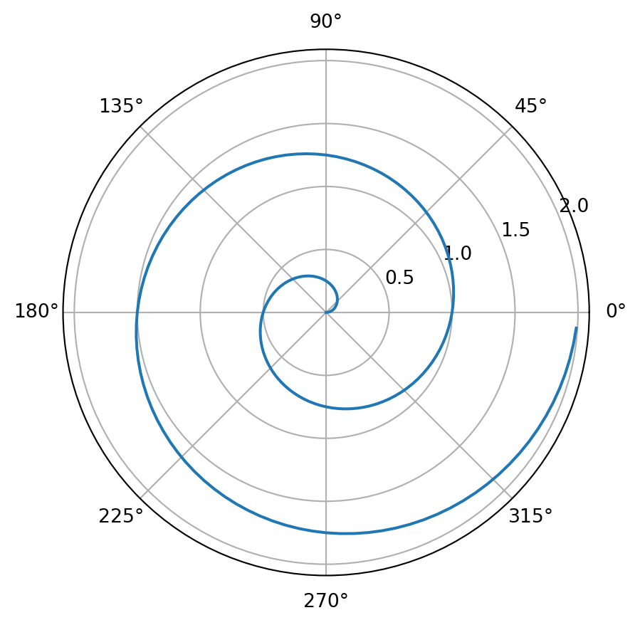
Machine learning (ML) is a branch of artificial intelligence (AI) focused on enabling computers and machines to imitate the way that humans learn, to perform tasks autonomously, and to improve their performance and accuracy through experience and exposure to more data.
Transformers (how LLMs work) explained visually | DL5 by 3Blue1Brown
A transformer, functioning as a perceptron within a multilayer large language model (LLM), utilizes self-attention to process input sequences.
Each word in the sentence “The best Costa Brava spot is …” can attend to all other words, allowing the model to capture contextual relationships and dependencies effectively.
This is accomplished through multi-head attention, where multiple attention mechanisms operate in parallel, enabling the model to analyze different aspects of the input simultaneously.
The repetition of these processes across layers enhances the model’s ability to refine its predictions, ultimately generating coherent and contextually relevant completions for the sentence.
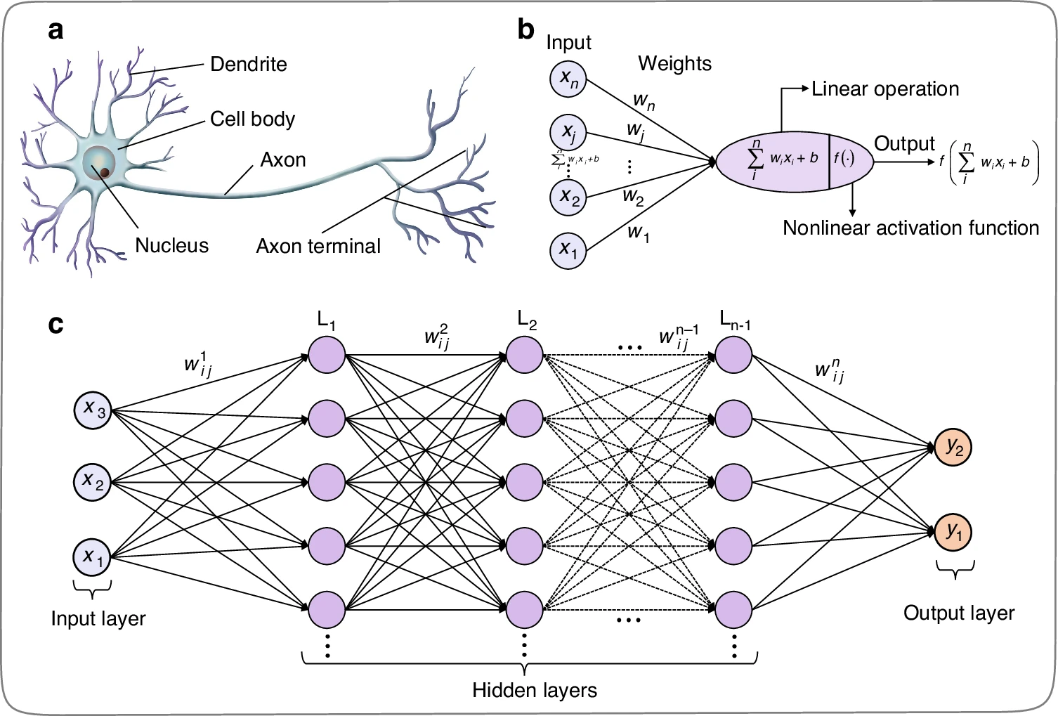
Each neuron computes a weighted sum of its inputs, adds a bias term, and applies an activation function. The output of a neuron can be represented as:
\[ y = f\left( \sum_{i=1}^{n} w_i x_i + b \right) \]
where ( w_i ) are the weights, ( x_i ) are the inputs, ( b ) is the bias, and ( f ) is the activation function.
Neuron structure and artificial neural network. a Structure of biological neurons. b Mathematical inferring process of artificial neurons in multi-layer perceptron, including the input, weights, summation, activation function, and output. c Multi-layer perceptron artificial neural network
Python is a versatile programming language widely used for coding Artificial Neural Networks (ANNs) and Machine Learning (ML) algorithms.
The Fourier series animation using Manim serves as an excellent example of how Python can be used to create complex visualizations and animations for mathematical concepts.
The Fourier series animation showcases Python’s ability to visualize complex mathematical concepts, which is crucial in ML for understanding data distributions, model architectures, and algorithm behavior.
Similarly, when working with ANNs and ML, you would use Python to create visualizations of your model’s architecture, training progress, and prediction results.
from manim import *

class FourierSeriesAnimation(Scene):
    def construct(self):
        # Create axes
        axes = Axes(
            x_range=[-2*PI, 2*PI, PI/2],
            y_range=[-2, 2, 1],
            axis_config={"color": BLUE},
        )

        # Create the original function (square wave)
        def square_wave(x):
            return np.sign(np.sin(x))

        original_func = axes.plot(square_wave, color=WHITE)

        # Define a list of colors for the approximations
        colors = [RED, GREEN, YELLOW, PURPLE, ORANGE]

        # Create Fourier series approximations
        approximations = []
        for n in range(1, 6):
            def fourier_series(x):
                return sum([(4 / ((2*k - 1) * PI)) * np.sin((2*k - 1) * x) for k in range(1, n+1)])

            approximations.append(axes.plot(fourier_series, color=colors[n-1]))

        # Add elements to the scene
        self.add(axes, original_func)

        # Animate the Fourier series approximations
        for approx in approximations:
            self.play(Create(approx), run_time=2)
            self.wait(1)

        self.wait(2)

# Render the scene
if __name__ == "__main__":
    scene = FourierSeriesAnimation()
scene.render()Quarto supports executable Python code blocks within markdown.
This allows you to create fully reproducible documents and reports—the Python code required to produce your output is part of the document itself, and is automatically re-run whenever the document is rendered.
import numpy as np
import matplotlib.pyplot as plt

r = np.arange(0, 2, 0.01)
theta = 2 * np.pi * r
fig, ax = plt.subplots(
  subplot_kw = {'projection': 'polar'}
)
ax.plot(theta, r)
ax.set_rticks([0.5, 1, 1.5, 2])
ax.grid(True)
plt.show()import numpy as np
import matplotlib.pyplot as plt
# Simulation parameters
T = 100 # Total time in ms
dt = 1 # Time step in ms
time = np.arange(0, T, dt)
# Neuron parameters
V_th = -50 # Spike threshold in mV
V_reset = -65 # Reset potential in mV
R = 1 # Resistance in MΩ
tau = 10 # Membrane time constant in ms
# Input current (constant for simplicity)
I = 1.5 # Input current in μA
# Initialize variables
V_m = V_reset * np.ones(len(time)) # Membrane potential array
spikes = [] # List to store spike times
# Simulation loop
for t in range(1, len(time)):
dV = (-(V_m[t-1] - V_reset) + R * I) / tau * dt # Update membrane potential
V_m[t] = V_m[t-1] + dV
# Check for spike
if V_m[t] >= V_th:
spikes.append(t) # Record spike time
V_m[t] = V_reset # Reset membrane potential after spike
# Plotting results
plt.figure(figsize=(10, 5))
plt.plot(time, V_m, label="Membrane Potential ($V_m$)", color='blue')
plt.plot(spikes, [V_th]*len(spikes), 'ro', label="Spikes") # Plot spikes as red dots
plt.axhline(V_th, color='black', linestyle='--', label="Spike Threshold")
plt.title("Membrane Potential of a Spiking Neuron")
plt.xlabel("Time (ms)")
plt.ylabel("Membrane Potential (mV)")
plt.legend()
plt.grid()
plt.show()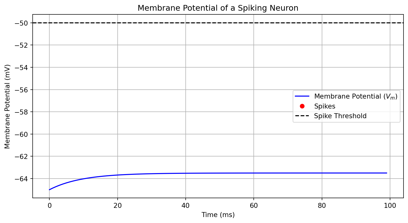
import numpy as np
import matplotlib.pyplot as plt
# Activation function: Sigmoid
def sigmoid(x):
return 1 / (1 + np.exp(-x))
# Derivative of the sigmoid function
def sigmoid_derivative(x):
return x * (1 - x)
# Input data (4 samples, 2 features)
X = np.array([[0, 0],
[0, 1],
[1, 0],
[1, 1]])
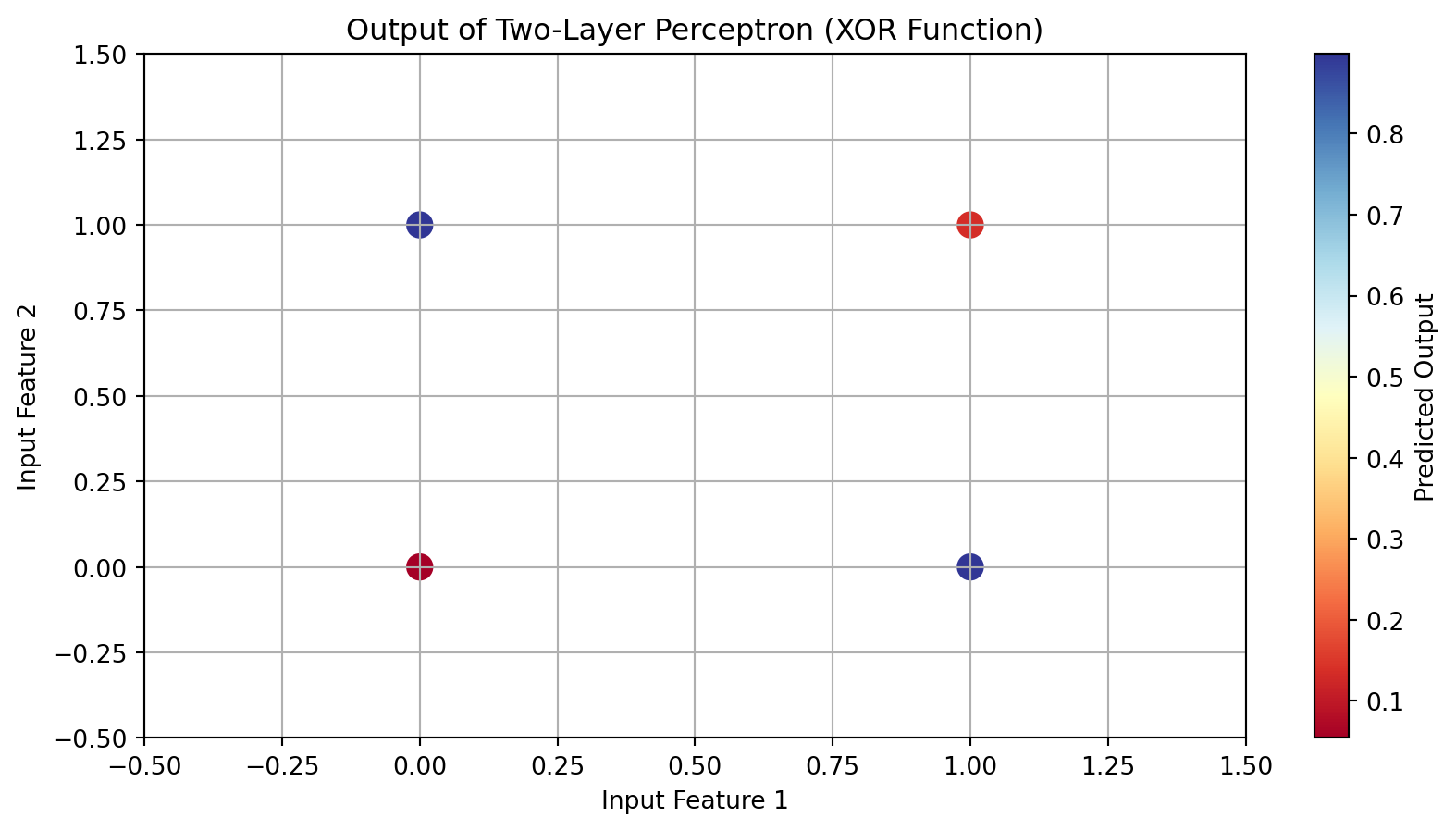
# Output data (XOR function)
y = np.array([[0],
[1],
[1],
[0]])
# Seed for reproducibility
np.random.seed(42)
# Initialize weights
input_layer_neurons = 2 # Number of input features
hidden_layer_neurons = 2 # Number of hidden neurons
output_neurons = 1 # Number of output neurons
# Weights between input layer and hidden layer
weights_input_hidden = np.random.uniform(size=(input_layer_neurons, hidden_layer_neurons))
# Weights between hidden layer and output layer
weights_hidden_output = np.random.uniform(size=(hidden_layer_neurons, output_neurons))
# Learning rate
learning_rate = 0.5
# Training the network
epochs = 10000
for epoch in range(epochs):
# Forward pass
hidden_layer_activation = np.dot(X, weights_input_hidden)
hidden_layer_output = sigmoid(hidden_layer_activation)
output_layer_activation = np.dot(hidden_layer_output, weights_hidden_output)
predicted_output = sigmoid(output_layer_activation)
# Backpropagation
error = y - predicted_output
d_predicted_output = error * sigmoid_derivative(predicted_output)
error_hidden_layer = d_predicted_output.dot(weights_hidden_output.T)
d_hidden_layer = error_hidden_layer * sigmoid_derivative(hidden_layer_output)
# Updating weights
weights_hidden_output += hidden_layer_output.T.dot(d_predicted_output) * learning_rate
weights_input_hidden += X.T.dot(d_hidden_layer) * learning_rate
# Final predictions after training
final_hidden_layer_activation = np.dot(X, weights_input_hidden)
final_hidden_layer_output = sigmoid(final_hidden_layer_activation)
final_output_layer_activation = np.dot(final_hidden_layer_output, weights_hidden_output)
final_predicted_output = sigmoid(final_output_layer_activation)
# Plotting results
plt.figure(figsize=(10, 5))
plt.scatter(X[:, 0], X[:, 1], c=final_predicted_output.flatten(), cmap='RdYlBu', s=100)
plt.title("Output of Two-Layer Perceptron (XOR Function)")
plt.xlabel("Input Feature 1")
plt.ylabel("Input Feature 2")
plt.colorbar(label='Predicted Output')
plt.grid()
plt.xlim(-0.5, 1.5)
plt.ylim(-0.5, 1.5)
plt.show()