Optimization essentials
The loss is a landscape
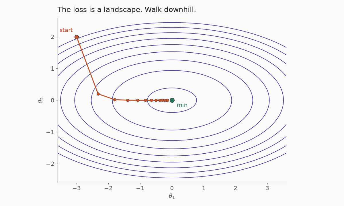
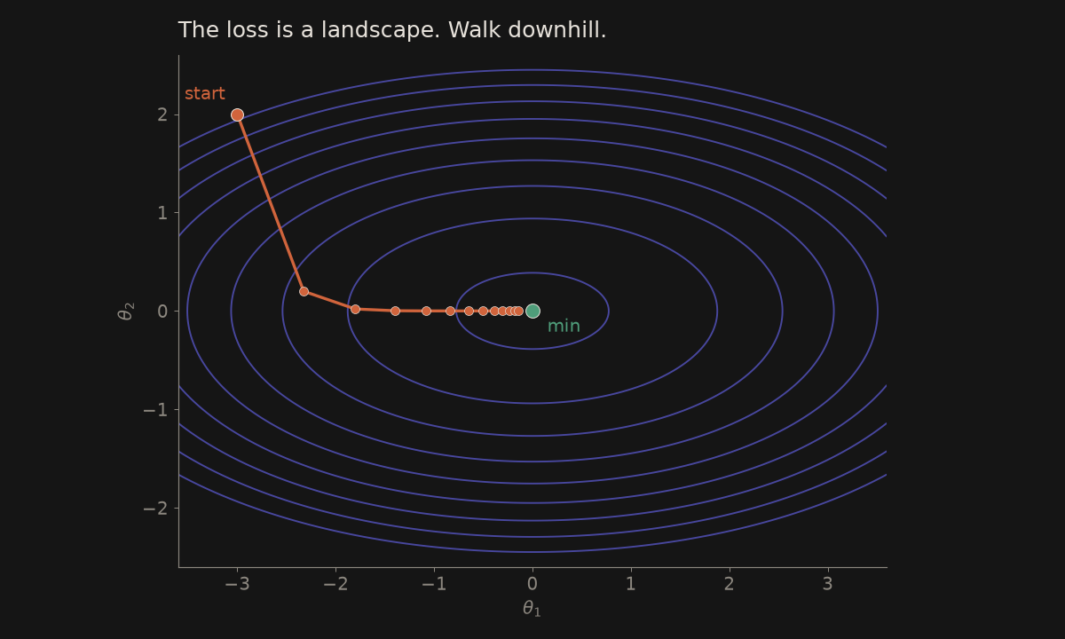
Training asks: which parameters make the error smaller? Write that error as a loss \(L(\theta)\). If you imagine \(L\) as height, the parameters sit on a landscape. A good model is a low point.
The formal question is \(\arg\min_\theta L(\theta)\): which \(\theta\) gives the smallest loss? See \(\arg\min\) on the symbols page. We rarely solve that in one shot. We walk downhill instead.
The gradient descent update
The gradient \(\nabla L\) (see calculus and the \(\nabla\) card) points uphill. A step the other way is
\[ \theta \leftarrow \theta - \eta\,\nabla L(\theta), \]
where \(\eta>0\) is the learning rate. A one-weight program that repeats this step is on The learning loop.
A tiny numeric example. Let \(L(w)=(w-3)^2\), so \(\nabla L=2(w-3)\). Start at \(w=5\) with \(\eta=0.1\) (the same toy loss as on the calculus page):
\[ w \leftarrow 5 - 0.1\times 4 = 4.6. \]
The loss falls from \(4\) to \(2.56\). Repeat, and \(w\) drifts toward \(3\), where the slope is zero.
The learning rate: too small or too big
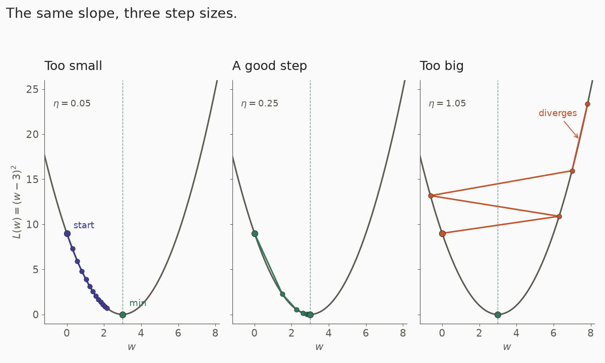
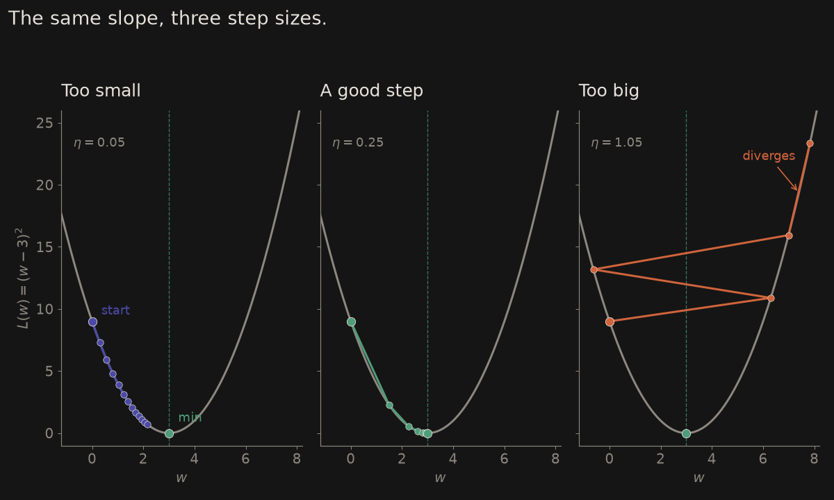
If \(\eta\) is too small, each step is a shuffle and training crawls. If \(\eta\) is too big, the step overshoots the valley and the loss can bounce or blow up. A good rate is large enough to make progress and small enough to settle.
Batch, stochastic, and mini-batch
The gradient is an average over examples.
- Batch (full-batch) uses every example at once. The path is smooth, but one step can be slow when the dataset is large.
- Stochastic gradient descent (SGD) uses one example (or one very small draw). The path is noisy, which is cheaper per step and can help the walk leave a shallow dip.
- Mini-batch takes a small group, often tens or hundreds of rows. This is the usual compromise: a stabler gradient than one row, still cheap enough to run on a GPU.
Momentum
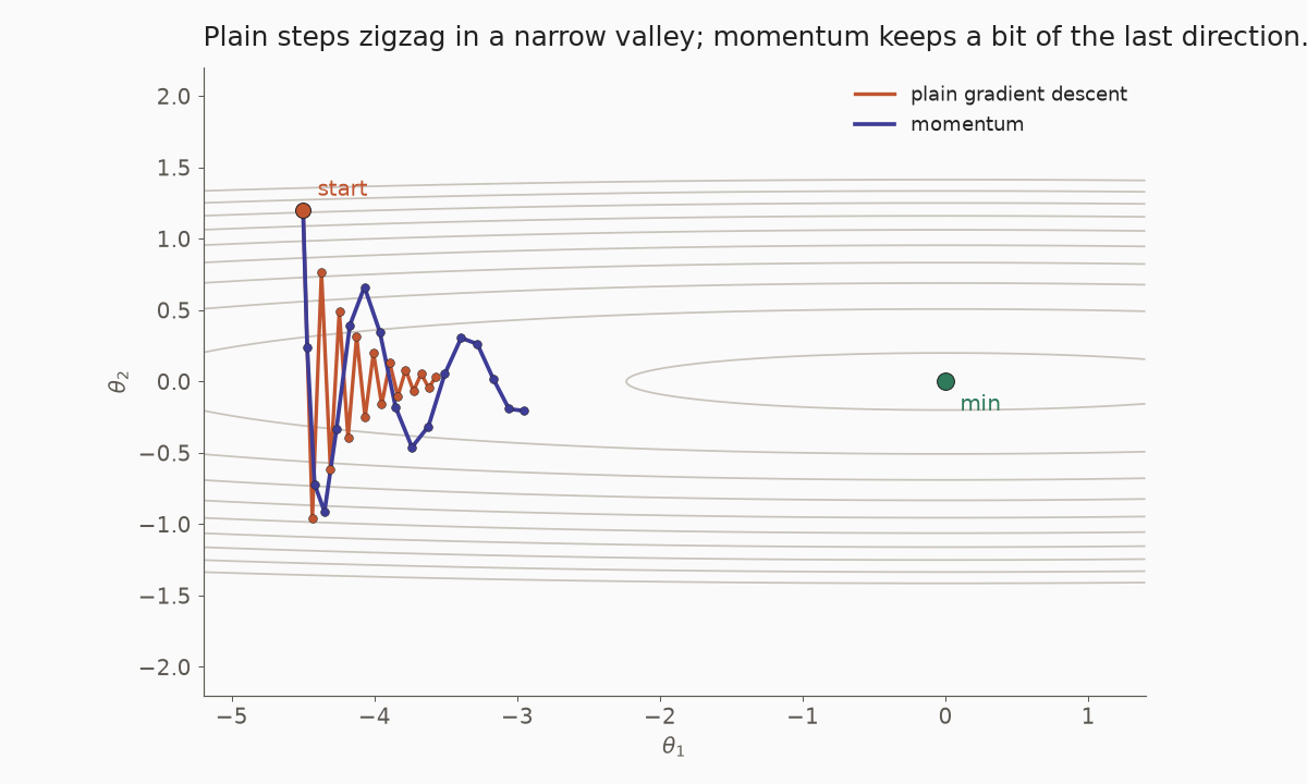
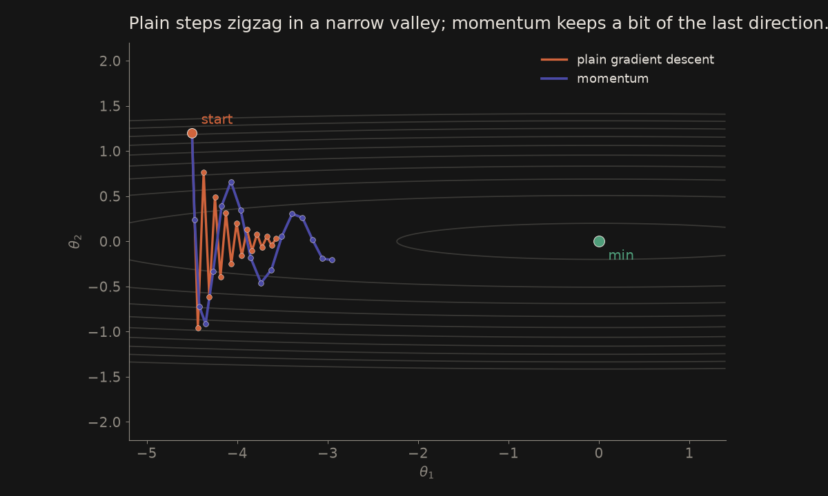
Plain steps can zigzag down a long, narrow valley: each step dives toward a wall, then back. Momentum keeps a running average of recent gradients and steps in that direction, so the walk builds speed along the valley and damps the zigzag.
Adam, in one idea
Adam (Kingma and Ba, 2014) is a very common default. The name is short for adaptive moment estimation. It keeps two running averages: one of the gradient (a momentum term) and one of the squared gradient (how large that parameter’s slopes have been). Parameters that have been seeing large, noisy slopes get a smaller effective step; quieter ones get a larger one. You still choose a base learning rate, but each parameter then adapts its own pace.
Local minima and saddle points
A local minimum is a dip that is lower than its neighbours, but not necessarily the lowest point on the whole landscape (the global minimum). A saddle point is a pass: uphill in some directions, downhill in others. In a high-dimensional loss, the walk can slow down near saddles, where the slope is almost flat. Mini-batch noise and methods such as momentum often help the walk keep moving.
A tiny NumPy walk
import numpy as np

# L(w) = (w - 3)**2, start at 5, learning rate 0.1
w, eta = 5.0, 0.1
for _ in range(5):
    grad = 2 * (w - 3)
    w = w - eta * grad
    print(w, (w - 3)**2)
# 4.6      2.56
# 4.28     1.6384
# 4.024    1.048576
# 3.8192   0.67108864
# 3.65536  0.4294967296
The slopes that feed this update come from the chain rule and, in a network, from the activation functions along the way.
See also
- The learning loop — the same update, with one weight, in a short program
- Calculus essentials — the slope, the chain rule, and one step of gradient descent
- ML math symbols, explained easy — \(\nabla\), \(\arg\min\)
- ANN: Activation functions — why some slopes vanish
- Maths for machine learning
References
- Diederik P. Kingma and Jimmy Ba, Adam: A Method for Stochastic Optimization, arXiv:1412.6980, 2014. https://arxiv.org/abs/1412.6980