The learning loop

A real example with one weight: taxi fare

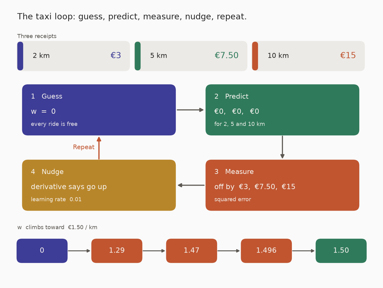
Price = w · kilometres, and w is unknown. You have three receipts: 2 km for €3, 5 km for €7.50, 10 km for €15. The true rate is €1.50 per kilometre, but nobody tells the model that.

The loop is the same one you will see in the code below.

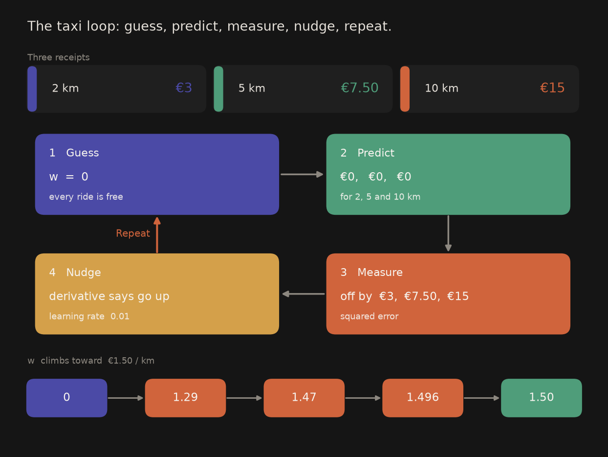
Guess: start with \(w = 0\) — every ride is free.
Predict: €0, €0, €0.
Measure: off by €3, €7.50, and €15.
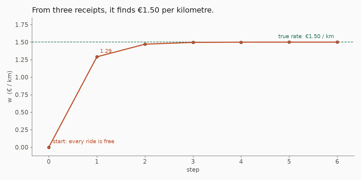
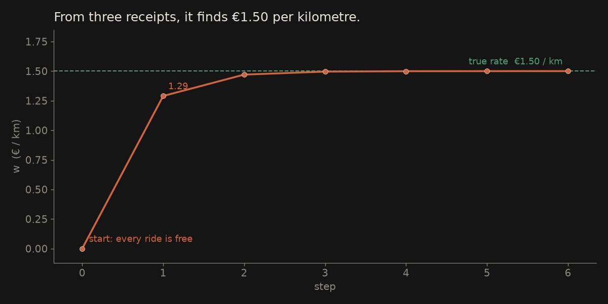
Nudge: the derivative says go up. With a learning rate of \(0.01\), \(w\) jumps to \(1.29\).
Repeat: \(1.47\), then \(1.496\), then about \(1.50\).

In three or four steps it has learned €1.50/km from three receipts. Nobody programmed the rate.

The taxi loop: guess, predict, measure the error, nudge w, and repeat, until w reaches €1.50 / km.

A bias (\(y = w\cdot x + b\)) would learn a pickup fee as well, the bit you pay before the metres start to run.

You can run this loop yourself in Lab#FU01-1: Taxi fare, pure Python. Lab#FU01-2 adds the pickup fee and compares your descent with scikit-learn.

After step	\(w\) (€/km)	Predictions	Loss
start	0.00	€0.00, €0.00, €0.00	96.75
1	1.29	€2.58, €6.45, €12.90	1.90
2	1.47	€2.94, €7.35, €14.71	0.037
3	1.496	€2.99, €7.48, €14.96	0.0007
4	1.499	€3.00, €7.50, €14.99	≈ 0

The fare per kilometre climbs from 0 to €1.50 in a few steps.

A real-world example: a spam filter

A spam filter is the same loop, with thousands of weights instead of one.

It starts by guessing that every word matters equally. It predicts spam or not for each email, then measures the error against emails that people have already marked as spam. It nudges the weights: “free money” goes up, “meeting tomorrow” goes down. Then it repeats, millions of times.

Google Maps arrival times and Netflix recommendations work the same way: guess, check against reality, adjust, repeat.

The simplest model

The simplest model is a single weight: \(y = w \cdot x\). We give it data where the true answer is \(w = 2\) (\(y\) is always \(2\times x\)) and watch it find that on its own.

The learning loop

Guess: start with \(w = 0\).
Predict: compute \(w \cdot x\) for each example.
Measure the error: how far off are the predictions? (squared error)
Nudge \(w\) in the direction that reduces the error (the derivative says which way).
Repeat.

Everyday example

You season a soup. Taste it: too little salt. Add a pinch, taste again. You do not dump the whole shaker — that would ruin it. That pinch is the learning rate; tasting and nudging, over and over, is how a model learns.

flowchart TD
  A[Start with a guess] --> B[Predict]
  B --> C[Measure the squared error]
  C --> D[Nudge the weight]
  D --> B

The code

The data is \(x=\{1,2,3,4\}\) and \(y=\{2,4,6,8\}\). The learning rate is \(0.01\), for \(20\) steps.

Java
Python

public class Learn {
    public static void main(String[] args) {
        double[] x = {1, 2, 3, 4};
        double[] y = {2, 4, 6, 8};   // y = 2 * x
        double w = 0;                // initial guess
        double lr = 0.01;            // learning rate (step size)

        for (int step = 0; step < 20; step++) {
            double grad = 0, loss = 0;
            for (int i = 0; i < x.length; i++) {
                double err = w * x[i] - y[i];
                loss += err * err;
                grad += 2 * err * x[i];   // derivative of err² with respect to w
            }
            loss /= x.length;
            grad /= x.length;

            w -= lr * grad;              // the learning step
            System.out.printf("step %d  w=%.3f  loss=%.4f%n", step, w, loss);
        }
    }
}

x = [1, 2, 3, 4]
y = [2, 4, 6, 8]   # y = 2 * x
w = 0.0            # initial guess
lr = 0.01          # learning rate (step size)

for step in range(20):
    grad = 0.0
    loss = 0.0
    for i in range(len(x)):
        err = w * x[i] - y[i]
        loss += err * err
        grad += 2 * err * x[i]   # derivative of err**2 with respect to w
    loss /= len(x)
    grad /= len(x)
    w -= lr * grad               # the learning step
    print(f"step {step}  w={w:.3f}  loss={loss:.4f}")

What you’ll see

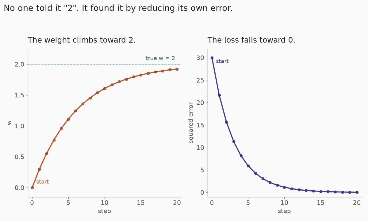
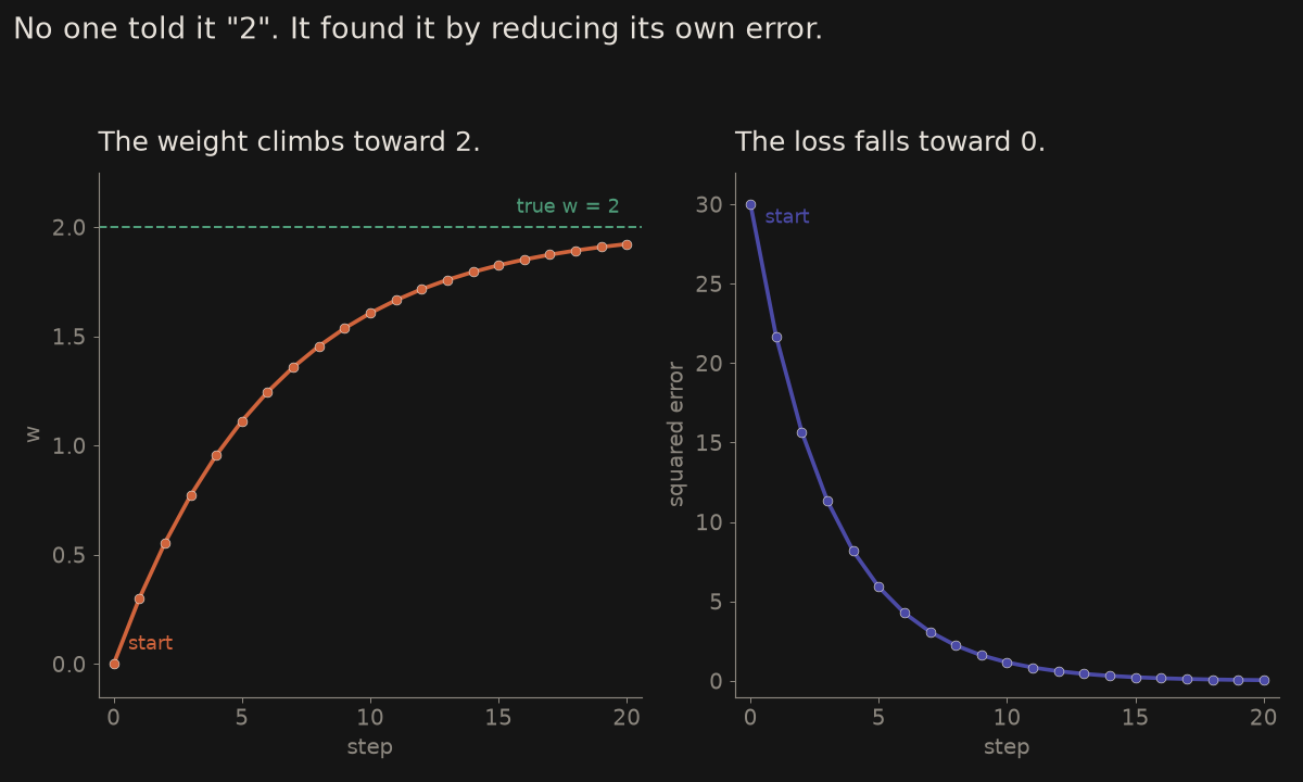
\(w\) starts at \(0\), jumps to \(0.3\) after the first step, then climbs toward \(2\) while the loss shrinks toward \(0\). That is learning: no one told it “\(2\)”, it found it by repeatedly reducing its own error.

A real run of the program above prints this (the loss on each line is the error before that step’s nudge):

step 0  w=0.300  loss=30.0000
step 1  w=0.555  loss=21.6750
step 2  w=0.772  loss=15.6602
step 3  w=0.956  loss=11.3145
step 4  w=1.113  loss=8.1747
...
step 18  w=1.909  loss=0.0863
step 19  w=1.922  loss=0.0624

After twenty steps, \(w\) is \(1.922\), already close to \(2\).

The weight climbs toward 2, and the squared error falls toward 0.

Try this

Change lr and run it again. The step size really matters.

lr = 0.001 — slow learning. After twenty steps, \(w\) is only \(0.522\) and the printed loss is still \(16.8927\).
lr = 0.1 — the first nudge overshoots: \(w\) jumps to \(3.000\), then zig-zags (\(1.500\), \(2.250\), \(1.875\), ) but it still converges, and faster than \(0.01\).
lr = 0.2 — it blows up. \(w\) goes \(6\), \(-6\), \(18\), \(-30\), and the loss keeps growing.

# lr = 0.1
step 0  w=3.000  loss=30.0000
step 1  w=1.500  loss=7.5000
step 2  w=2.250  loss=1.8750
step 3  w=1.875  loss=0.4688

# lr = 0.2
step 0  w=6.000  loss=30.0000
step 1  w=-6.000  loss=120.0000
step 2  w=18.000  loss=480.0000

The nudge itself is the same idea as on the optimization page: \(w \leftarrow w - \eta\nabla L\). The gradient says which way.

Why this is so relevant, and why we say a machine is learning

This little loop is so relevant because it is the same loop behind every neural network: an MNIST classifier, a large language model, all of them. Only the scale changes — more weights, more data, a longer chain. The idea does not.

Why do we say the machine is learning? Nobody programmed \(w = 2\). We did not write the rule y = 2 * x. The program started from a wrong guess and improved its own performance from data and experience, by reducing its error, step after step.

Tom Mitchell put it this way in 1997:

A computer program is said to learn from experience E with respect to some class of tasks T and performance measure P, if its performance at tasks in T, as measured by P, improves with experience E.

Here the task \(T\) is to predict \(y\) from \(x\), the performance \(P\) is the squared error (smaller is better), and the experience \(E\) is the four examples. After twenty steps, \(P\) has improved. So we call it learning.

Everyday example

You learn to throw a dart, or to ride a bike, in the same way: you miss, you correct, you try again. Nobody hands you a finished list of rules. The machine is doing that, with a number \(w\).

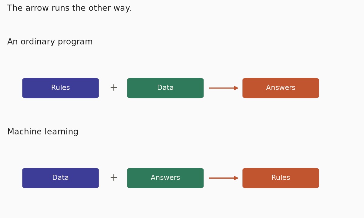
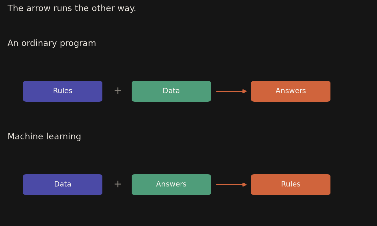
An ordinary program works like this: you write the rules, you give it data, and it produces answers. Machine learning flips the arrow: you give it data and the answers, and it finds the rules.

An ordinary program is rules plus data, giving answers. Machine learning is data plus answers, giving rules.

Next step: a bias

Next step would be adding a bias: \(y = w\cdot x + b\). Now two numbers have to be learned, not one, but the loop does not change: predict, measure the error, nudge each parameter, repeat. That is Lab#FU01-2: Taxi fare, NumPy and scikit-learn.

References

Tom M. Mitchell, Machine Learning, McGraw-Hill, 1997. The definition above is from Chapter 1, “Well-posed learning problems”.

A real example with one weight: taxi fare

A real-world example: a spam filter

The simplest model

The learning loop

The code

What you’ll see

Try this

Why this is so relevant, and why we say a machine is learning

Next step: a bias

See also

References