Attention Is All You Need

A reader’s guide to the 2017 paper

A paper that opened a door

Attention Is All You Need (Vaswani, Shazeer, Parmar, Uszkoreit, Jones, Gomez, Kaiser and Polosukhin, 2017) is the paper that introduced the Transformer. This page is a reader’s guide: what problem it solved, how the architecture is put together, what the experiments showed, and how to walk through the sections without getting lost.

The PDF is on arXiv (1706.03762). It also appeared at NeurIPS 2017; the official proceedings PDF is the one linked from our resources.

The story that leads to the paper — Bahdanau, Luong, then self-attention as the foundation — is in The evolution of attention. A tiny block, worked with integers you can add by hand, is in Transformer by hand. Here we stay close to the paper itself.

The problem it solved

Before this paper, the strongest models for translation and other sequence tasks were recurrent: LSTMs and GRUs, usually in an encoder-decoder, often with an attention mechanism on top. A recurrent net reads one token, then the next, then the next. Position \(t\) has to wait for position \(t-1\). That queue is hard to parallelise, and it gets worse as the sequence gets longer.

Attention was already helping — a decoder could look back at the source instead of trusting a single summary vector. But in almost every successful model, attention still sat on top of a recurrent backbone. The bottleneck of one-token-after-another training was still there.

Everyday example

A recurrent net is a queue at a counter: person 2 cannot be served until person 1 has finished. The Transformer is a room in which everyone can be seen at once. To know who arrived first, you still need a ticket with a number — that is the positional encoding.

The key idea

The title is the claim. If attention is doing the real work, why keep the recurrence at all?

The Transformer dispenses with recurrence and convolutions entirely. It is built from attention, position-wise feed-forward layers, residual connections, layer normalisation, and a signal for word order. Because every position can be processed together, training can use a GPU properly. Reading the input is parallel; writing the output is still one token at a time.

The architecture

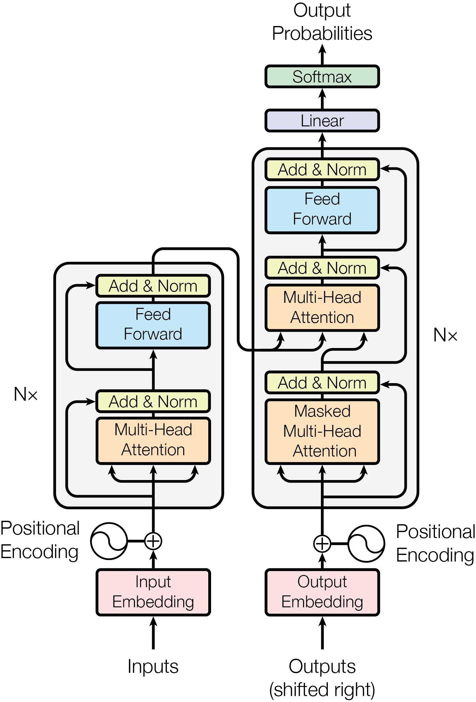
The paper keeps the usual encoder-decoder shape, built for translation: the encoder reads the source and builds a representation of it; the decoder writes the target, one token at a time, looking at that representation and at what it has already written.

flowchart TD
  SRC[Source tokens] --> PE1[Positional encoding]
  PE1 --> ENC[Encoder stack: 6 layers]
  ENC --> EDA[Encoder-decoder attention]
  TGT[Tokens written so far] --> PE2[Positional encoding]
  PE2 --> MSK[Masked self-attention]
  MSK --> EDA
  EDA --> FF2[Feed-forward]
  FF2 --> OUT[Next-token probabilities]

In the base model, both stacks have \(N = 6\) layers, and every sub-layer writes vectors of size \(d_{\text{model}} = 512\).

Encoder and decoder stacks

Each encoder layer has two sub-layers: multi-head self-attention, then a position-wise feed-forward network. Around each sub-layer the paper puts a residual connection, then layer normalisation:

\[ \operatorname{LayerNorm}\bigl(x + \operatorname{Sublayer}(x)\bigr) \]

The residual is a skip: the original \(x\) is added back, so the sub-layer only has to learn a change, not the whole signal again.

Each decoder layer has three sub-layers. The first is masked self-attention over the tokens written so far. The second is encoder-decoder attention: the decoder asks questions, and the answers come from the encoder. The third is the same kind of feed-forward network as in the encoder. Residuals and layer norm wrap each of the three, just as in the encoder.

Scaled dot-product attention

This is the attention formula the paper uses, and the one we unpacked in The evolution of attention:

\[ \operatorname{Attention}(Q, K, V) = \operatorname{softmax}\!\left(\frac{QK^{\top}}{\sqrt{d_k}}\right)V \]

Queries, keys and values are packed into matrices. The scaling \(1/\sqrt{d_k}\) stops the dot products growing with the key size and flattening the softmax. The paper contrasts this with Bahdanau’s additive attention: the scores are similar in spirit, but a dot product is a much better fit for fast matrix multiplication on a GPU.

Multi-head attention

One attention can focus on one kind of relationship. The paper runs \(h\) attentions in parallel — the heads — each with its own learned projections of \(Q\), \(K\) and \(V\). The heads are concatenated and projected back to \(d_{\text{model}}\).

In the base model there are \(h = 8\) heads, and each head uses \(d_k = d_v = 64\). Because each head is narrower, the total cost stays close to that of a single full-width head.

Everyday example

A team of readers looks at the same page. One tracks who did what, another tracks what it refers to, another tracks nearby words. Then you put their notes together. That is multi-head attention: several looks, then one combined result.

The Transformer uses this block in three places:

Encoder self-attention. Every source position can look at every source position.
Decoder self-attention, with a mask. Each target position can look only at itself and at earlier target positions, never at the future.
Encoder-decoder attention. Each target position can look at every source position. This is the old “look back at the letter” step, now with the same multi-head machinery.

Masking

The decoder must not cheat. When it predicts token \(i\), it may use only tokens before \(i\). The paper enforces that inside attention: illegal scores are set to \(-\infty\) before the softmax, so their weights become zero. The output embeddings are also shifted by one position. Together, those two devices keep the decoder auto-regressive: it writes one token, adds it to the context, and writes the next.

Positional encoding

Because the model reads all the tokens at once, it does not naturally know the order. The paper adds a positional encoding to the embeddings at the foot of both stacks, with the same width \(d_{\text{model}}\), so the two can be summed.

The version they use is a fixed pattern of sines and cosines:

\[ \begin{aligned} PE_{(pos, 2i)} &= \sin\bigl(pos / 10000^{2i/d_{\text{model}}}\bigr) \\ PE_{(pos, 2i+1)} &= \cos\bigl(pos / 10000^{2i/d_{\text{model}}}\bigr) \end{aligned} \]

Even dimensions get a sine, odd dimensions a cosine, and the wavelengths form a geometric progression. They also tried learned positional embeddings and found nearly the same quality (Table 3, row (E)). They kept the sinusoids because the pattern may extend to lengths the model did not see in training.

Feed-forward, residuals and layer norm

The feed-forward network is the same idea as in Transformer by hand: two linear maps with a ReLU in between, applied to each position with the same weights.

\[ \operatorname{FFN}(x) = \max(0, xW_1 + b_1)W_2 + b_2 \]

In the base model the inner width is \(d_{ff} = 2048\). The recipe is shared across positions, but not across layers: each layer has its own \(W_1\) and \(W_2\).

The residual plus layer norm around every sub-layer is what keeps a stack of six (or more) trainable. You can think of the skip as a handrail: the main signal can still get through if a sub-layer does something awkward.

A tiny taste: positional encoding, in the page

The cell below builds a small table of sinusoidal encodings, with \(d_{\text{model}} = 8\) and four positions, \(0\) to \(3\). Position \(0\) is \(0, 1, 0, 1, \ldots\) — sine of \(0\) and cosine of \(0\). At position \(1\), the first two numbers are just \(\sin 1\) and \(\cos 1\). Press Run after you change a setting if you like.

The editor is live Python in the browser. It uses only NumPy.

Training and results

The paper trains on standard WMT 2014 translation data. English-to-German uses about 4.5 million sentence pairs and a shared byte-pair vocabulary of about 37,000 tokens. English-to-French uses a much larger set, 36 million sentences, and a 32,000 word-piece vocabulary. Batches are grouped by length, at about 25,000 source tokens and 25,000 target tokens each.

Everything ran on one machine with eight NVIDIA P100 GPUs. The base model (\(d_{\text{model}} = 512\), eight heads, about 65 million parameters) was trained for 100,000 steps, about 12 hours. The big model (\(d_{\text{model}} = 1024\), sixteen heads, about 213 million parameters) was trained for 300,000 steps, 3.5 days. The optimiser is Adam, with a learning-rate schedule that warms up for 4,000 steps and then decays.

On the WMT 2014 test sets, Table 2 — and the abstract — report 28.4 BLEU for English-to-German and 41.8 BLEU for English-to-French, for the big model. The English-to-German result improved on the previous best, including ensembles, by more than 2 BLEU. (The prose in §6.1 writes 41.0 for the English-to-French score; the table and the abstract say 41.8.)

The paper also shows that the same architecture can be used for English constituency parsing, with both large and limited training data. That is the last experiment, not a second translation test.

Why it mattered

The headline at the time was translation quality at a fraction of the previous training cost, with a model that could finally use a GPU in parallel. The longer consequence is the shape of almost everything that followed.

The encoder stack is the ancestor of BERT and the family of models that read a text and build a representation of it. The decoder, taken on its own and trained to predict the next token, is the ancestor of GPT and the chat models we use now. The original paper is an encoder-decoder, built for translation. The two halves were later used separately, at a much larger scale.

The evolution of attention picks up what came next on the attention formula itself: linear attention, then FlashAttention. This page stops at the 2017 design.

How to read the paper

A good path is to follow the paper’s own sections, with a question in mind for each.

Introduction. Why recurrence is a queue, and why attention-on-top-of-an-RNN is not enough.
Background. Self-attention already existed; the claim is a model that relies on it entirely, with no recurrence and no convolution.
Model architecture. This is the heart. Read 3.1 (the stacks, residual plus layer norm, the mask) and 3.2 (scaled dot-product, multi-head, the three uses) slowly. 3.3 is the feed-forward network you have already computed in Transformer by hand. 3.4 is embeddings and the shared softmax weights. 3.5 is the sinusoids, which the cell above makes concrete.
Why self-attention. A comparison of cost, parallel work, and the path length between distant tokens. Useful once the architecture is in your head; it can wait until a second pass if you prefer.
Training. Data, hardware, Adam and the warmup, dropout and label smoothing. Skim it the first time; come back when you want to reproduce something.
Results. Table 2 is the headline (28.4 and 41.8). Table 3 is the ablation: what happens if you change the number of heads, \(d_k\), the depth, or the positional encoding. The parsing experiment is in the same section.
Conclusion. Short. The last paragraph is the claim again: attention is enough.

Two careful readings that walk through the same material with code and pictures, if you want a companion: The Annotated Transformer (Harvard NLP) and The Illustrated Transformer (Jay Alammar). They are guides to the paper, not a substitute for it.

In one table

Piece	What it does in the paper
Encoder stack	\(N = 6\) layers; self-attention, then a feed-forward network; residual plus layer norm around each
Decoder stack	\(N = 6\) layers; masked self-attention, encoder-decoder attention, then a feed-forward network
Scaled dot-product	\(\operatorname{softmax}(QK^{\top}/\sqrt{d_k})V\)
Multi-head attention	\(h = 8\) heads in the base model, \(d_k = d_v = 64\), then concatenate and project
Masking	Illegal decoder scores are set to \(-\infty\) before softmax, so the future cannot leak
Positional encoding	Sine and cosine, added to the embeddings; learned embeddings were almost as good
Feed-forward	\(\max(0, xW_1 + b_1)W_2 + b_2\), width \(d_{ff} = 2048\) in the base model, position-wise
Training	WMT 2014; Adam with a 4,000-step warmup; base model about 12 hours, big model 3.5 days, on eight P100 GPUs
Headline results	Table 2: 28.4 BLEU (EN-DE) and 41.8 BLEU (EN-FR), big model

FAQ

Does a Transformer write the whole translation in parallel?

No. It can read the source in parallel, and training can exploit that. While writing, it still predicts one token at a time, adds that token to the context, and predicts again. The mask is there to keep that rule.

Is the Transformer only an encoder-decoder?

The 2017 model is an encoder-decoder, because it was built for translation. Later work often uses only the decoder (as in GPT-style models) or only the encoder (as in BERT-style models). The blocks inside are the same family.

Why divide by \(\sqrt{d_k}\)?

Without the scaling, the dot products tend to grow with the size of the key, and softmax becomes a sharp spike that is hard to train. Section 3.2.1 of the paper, and the everyday version in The evolution of attention, both start from that observation.

Did they invent attention?

No. Attention, including the encoder-decoder kind, was already in use. The paper’s claim is that attention is enough: you can drop the recurrent backbone and still get a better, more parallel model. That is the “all you need”.

The English-to-French BLEU is 41.8 in the table. Why does §6.1 say 41.0?

The abstract and Table 2 report 41.8. The paragraph in §6.1 writes 41.0. We have not tried to decide which line is the intended one; when we quote a headline figure we follow the table and the abstract, and we note the prose here so you can see both when you read the paper.